Fast multipole method
Note · 12 November 2026 · Computer science › Algorithms
The Barnes–Hut algorithm makes the N-body problem cheap, as long as one percent of error is good enough. A graph layout can live with that. Electrostatics in a protein, or an integral equation in engineering, needs six to twelve correct digits. Barnes–Hut can only reach them by opening more and more cells, until it is slower than the direct sum.
The figure computes the same 4000 potentials three ways. Barnes–Hut at θ = 0.1 reaches an error of and takes 1.6 s, longer than the 1.3 s of the exact direct sum. The fast multipole method (FMM) reaches in 82 ms. This note shows how.
The idea: let boxes talk to boxes
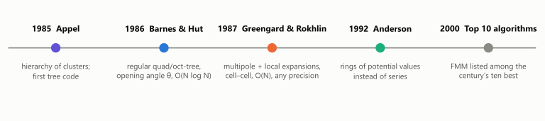
In 1986, Barnes–Hut had two limits. A far cell acted only through its total mass, so accuracy came only from opening cells. Each body also walked the tree on its own, which kept a factor.
Greengard and Rokhlin removed both limits in 1987 (Greengard and Rokhlin 1987). Their first move keeps more information about a far box: not one number, but a series of terms. Each extra term buys a fixed number of digits. Their second move lets a far box act on a whole target box at once, through a second series centred on the target. Then a box costs the same, however many bodies it holds, and the total work becomes .
The method needs four steps:
- describe every box by a multipole expansion of its charges;
- convert far multipoles into a local expansion around each target box;
- decide which boxes translate to which, with the interaction list;
- organise all of it as an upward and a downward pass over the tree.
This note works in 2D with the potential , where points are complex numbers . That is the setting of the 1987 paper. In 3D the series are spherical harmonics, but the four steps stay the same.
Step 1: one box as one series
The charges at in a box with centre produce, at any point further away than all of them, The coefficients are the multipole moments of the box. Computing them from the particles is the operator P2M.
Greengard and Rokhlin bound the error after terms by where is the radius of a circle around that holds all the charges. So the error falls geometrically with , and it falls faster further away.
In the figure, the dashed circle is that radius. With p = 0 only the total charge is left, which is what Barnes–Hut uses: the error is even four box widths away. With p = 4 it is at two box widths, and with p = 12 it is . Inside the circle the series diverges at every : no number of terms helps there.
- Why does the error pattern stay round, although the box is square?
- How many terms does one extra digit cost at two box widths, and at four?
Step 2: collect the far field in a local series
A multipole series still has to be evaluated once for every target body. The second idea removes that cost. Around the centre of a target box, the field of a far box is smooth, so it has a Taylor series: The operator M2L computes the directly from the far box’s multipole moments , without touching its particles. With the source centre relative to the target centre, Local series from many far boxes simply add up. One set of coefficients then carries the whole far field of a target box, and every body in the box reads its potential from it.
In the figure the two boxes are five box widths apart. With p = 2 the worst error inside the target box is . With p = 8 it is , and with p = 16 it reaches the rounding error of double precision. The good region is a disc around the target. It grows with but never reaches the source box.
Step 3: who talks to whom
The FMM uses a quadtree of uniform depth : level has boxes. Two boxes on the same level are well separated when they do not touch. For a target box, the space splits into three parts:
- its 8 touching neighbours, plus itself, are the near field, summed particle by particle at the finest level;
- its interaction list holds the children of its parent’s neighbours that do not touch it, at most 27 boxes, and each sends one M2L;
- everything further away was already well separated from the parent, so the parent’s local series carries it.
At depth 3 one leaf needs 7 + 27 translations and 9 near boxes, out of 64 leaves. At depth 4 it needs 7 + 27 + 27 out of 256, and at depth 6 7 + 4 × 27 out of 4096. The work grows by 27 per level, while the number of leaves grows by a factor of 4. Click other leaves: boxes at the edge have shorter lists.
Step 4: the two passes
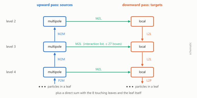
The four ideas become one algorithm with five operators.
| Operator | From → to | Pass |
|---|---|---|
| P2M | particles → multipole of a leaf | upward |
| M2M | four child multipoles → parent multipole | upward |
| M2L | multipole of a listed box → local series of the target | downward |
| L2L | parent local series → child local series | downward |
| L2P | local series → potential at each particle, plus the near field | downward |
The upward pass starts with P2M at the leaves, then shifts the multipoles up one level at a time with M2M. The shift is exact up to the truncation at terms, so no particle is visited twice. The downward pass starts at level 2 with the M2L translations. On each finer level, a box takes its parent’s series through L2L and adds the translations from its own list. At the leaves, L2P evaluates the series at the particles and adds the direct near-field sum.
Why the cost is O(N)
- Let each leaf hold about particles, so there are about leaves and boxes in all.
- Every box does at most 27 M2L translations of cost , one M2M and one L2L. That is in total.
- The near field costs terms per particle, so in total. P2M and L2P cost per particle.
- The total, , is linear in for a fixed and leaf size. The best leaf size grows like , and then the cost is .
- The precision sets . The closest M2L partners are two box widths apart, so in the worst case each term gains about digits. In the benchmark below the measured gain is about 0.45 digits per term: 7 digits for 16 more terms.
Performance analysis
All three methods run in the same JavaScript. The charges are uniform random unit charges, and the error is the largest potential error, relative to the largest potential. The leaf holds about 16 to 31 particles. The button measures again on your machine, up to N = 8000.
| N | direct | Barnes–Hut θ = 0.5 | FMM p = 8 | FMM p = 16 |
|---|---|---|---|---|
| 1000 | 89 ms | 24 ms, error | 19 ms, | 21 ms, |
| 4000 | 1.3 s | 208 ms, | 126 ms, | 115 ms, |
| 16000 | 22.8 s | 821 ms, | 249 ms, | 322 ms, |
- At N = 16,000 the FMM with 8 terms is 92 times faster than the direct sum. It is also 3 times faster than Barnes–Hut, while its error is 500 times smaller.
- Going from 8 to 16 terms costs little here, because the near field dominates the time at these sizes. The digits come almost for free, as the accuracy wall shows.
- At N = 500 the FMM is not faster than the direct sum (27 ms against 22 ms). The tree and the translations have a fixed cost, so small problems should stay direct.
- The time grows in steps, not smoothly: the tree depth is a whole number, and each new level changes the leaf size by a factor of 4.
1992: Anderson’s rings
- Greengard and Rokhlin derived the five operators for one kernel, the log potential. Every new kernel needs a new derivation, and in 3D the algebra of spherical harmonics is heavy.
- Anderson removed the series algebra (Anderson 1992). A potential that is harmonic outside a circle is fixed by its values on that circle. So each box stores the potential at points on a ring instead of series coefficients.
- An outer ring rebuilds the potential outside the circle and plays the part of a multipole expansion. An inner ring rebuilds it inside and plays the part of a local expansion. The only kernel the method ever evaluates is the potential itself.
- This is the variant of the Scientific Computing 2 course (worksheet 5). anderson_rings.py checks both rings for 50 unit charges, with the target about 4.7 box widths away:
| M (ring points K = 2M+1) | 2 | 6 | 10 | 14 |
|---|---|---|---|---|
| outer-ring error | ||||
| inner-ring error (exact ring values) |
- In 2000 the FMM was listed among the ten algorithms of the 20th century with the greatest influence on science and engineering (Dongarra and Sullivan 2000).
Code
- fmm-figure.html: the figure of this note. It contains a complete 2D FMM in JavaScript, with Barnes–Hut and the direct sum for comparison, and produced every number above.
- fmm_2d.py: the same algorithm in Python, with the five operators as separate methods.
- anderson_rings.py: Anderson’s rings, cleaned from the course solution. The course weighted the ring sum by , which is correct only for ring radius ; the vault code uses .
Further reading
- Greengard and Rokhlin’s paper (Greengard and Rokhlin 1987) is short and readable. Its Lemmas 2.1 to 2.5 are the five operators of this note.
- Jeffrey Heer, The Barnes-Hut Approximation (Heer 2017) ends where this note begins, and points to the FMM for higher precision.
Links:
- Barnes–Hut algorithm — the predecessor: particle–cell interactions and only the total-charge term.
- Multigrid method — the other hierarchical solver. Multigrid works on a differential equation and its grid levels; the FMM works on the integral form and its box levels.
- Molecular dynamics — electrostatics is the long-range force that MD cannot cut off.
- Algorithms and data structures — the hall of fame there lists the FMM.
References:
- Scientific Computing 2, TUM (2020), lecture 5 and worksheet 5.