Barnes–Hut algorithm
Note · 12 November 2026 · Computer science › Algorithms
A galaxy, a protein in water and a drawing of a social network share one computation. Every point pulls or pushes every other point. A simulation of any of them needs the sum of all those forces, at every time step. This is the N-body problem.
The figure runs two discs of stars into each other, with gravity computed by the Barnes–Hut algorithm. Switch to the direct sum and the time per force evaluation jumps. Raise N to 5000 and the animation stalls. Go back to Barnes–Hut and it runs again. This note explains where that difference comes from.
The direct sum
The force on body is a sum over all the other bodies. With the gravitational constant set to 1, it is The small softening length keeps the force finite when two bodies come very close.
Each dotted line in the figure is one term. One body needs terms, and all bodies together need pairs. Twelve points give 66 pairs, and 120 points give 7140. A million stars give pairs per time step, and a simulation needs thousands of steps.
How can we do better?
The idea: a far group acts like one body
Before 1985, simulations either paid for every pair or solved the Poisson equation for the potential on a grid with fast Fourier transforms. The grid is fast, but its spacing sets the resolution. Galaxies and molecules cluster, so most of a grid is empty while the dense regions are under-resolved.
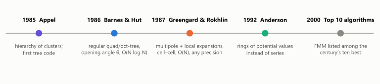
Appel grouped nearby bodies into a hierarchy of clusters and let a distant cluster act as a single body (Appel 1985). His tree followed the bodies, so its shape was irregular and its error was hard to predict. In 1986 the astronomers Josh Barnes and Piet Hut replaced it with a regular subdivision of space and one simple rule (Barnes and Hut 1986).
The key idea is to replace a group of distant bodies with their total mass at their centre of mass. That costs a small error, and it brings the work down from to .
The method needs a map of space that groups the bodies. In two dimensions this is a quadtree: a square is split into four equal quadrants, and each quadrant again, as far as needed. In three dimensions an octree splits a cube into eight. The algorithm has three steps:
- build the quadtree;
- compute the mass and the centre of mass of every cell;
- estimate the force on each body by walking the tree.
Step 1: build the quadtree
The tree starts as one root cell that covers the whole domain. The first point simply goes into the root. A second point would share the cell, so the root splits into four children and each point moves into its own quadrant. Every later insertion walks down from the root to the leaf that contains it, and splits that leaf if it is occupied. After 17 points the tree is already 5 levels deep near the clusters. With all 120 points it has 207 cells and depth 8.
- The figure stops splitting at one point per leaf, as Barnes and Hut did. Practical codes stop at a leaf size of about 8 to 32 points, which makes the tree shallower and the leaf sums cheaper. The vault code and the benchmark below use 8.
- For uniformly spread points the depth grows like . For clustered points it grows with the density contrast instead, because the tree refines only where points are.
- Each insertion costs one walk from the root, so the whole build costs . Parallel codes often build the tree differently: they sort the points along a space-filling curve, which puts every cell’s points next to each other in memory.
Step 2: compute the centres of mass
Every cell needs its total mass and its centre of mass: A parent needs its children first, so the pass starts at the deepest leaves. It then merges level by level and ends at the root, which holds all the mass at the overall centre of mass. Each cell is visited once, so this step costs .
Step 3: estimate the force
To find the force at a point, the walk starts at the root. A cell of width whose centre of mass is at distance is far enough when The walk then uses the cell’s total mass at its centre of mass and does not look inside. Otherwise it opens the cell and repeats the test on the children. A leaf that is still too close is summed point by point. The opening angle is the one parameter of the method.
At θ = 0 no cell is ever far enough, and the walk becomes the direct sum: 120 terms and no error. At θ = 0.5 the probe uses 21 cells and 21 single points, and the force error is 0.7 %. At θ = 1 only 18 terms are left, and the error at this probe jumps to 33 %. Try it yourself:
- Move the probe into a cluster. How does the number of single points change?
- Put it in empty space. Why do nearly all the terms become cells?
- At θ = 1, the grey and violet arrows can point in quite different directions. Which cells cause that?
The force on every body is such walks, one per body. That is the step that makes the method .
Why the cost is N log N
- Take a target and one level of the tree, where all cells have width . The walk accepts a cell at this level only if two tests hold. Its parent was too close, at . The cell itself is far enough, at .
- The accepted cells therefore sit in a ring of radius about to . Such a ring holds about cells in 2D, and about in 3D.
- There are about levels, so one target costs terms. All targets together cost .
- A smaller θ buys accuracy with work. Halving θ multiplies the work by about 4 in 2D and about 8 in 3D.
How large is the error?
- Expand the potential of the bodies in one cell around a centre , at a target distance much larger than the cell:
- The dipole moment is zero when is the centre of mass. The first neglected term is then the quadrupole, and the relative error of one cell is about .
- The errors of many cells partly cancel, because their quadrupoles point in different directions. In the benchmark below, θ = 0.5 cuts the mean force error to 0.9 %, from 5.5 % at θ = 1.
- The mean hides the worst case. The largest error per body is 2 to 9 times the mean, and the ratio grows with θ. It falls on bodies where large pulls from several sides nearly cancel.
- The course code put the pseudo-particle at the geometric cell centre instead of the centre of mass. That keeps the dipole term, and for 2000 uniform bodies it gave a 13–28 % larger potential error at the same θ.
Performance analysis
The figure compares the direct sum with Barnes–Hut at three values of θ, in the same JavaScript code. The points are uniform random in the unit square, the leaf size is 8, and the softening is 0.3 times the mean spacing. The error of one body is the length of its force error, divided by the mean force over all bodies. The button measures again on your own machine, up to N = 4000.
| N | direct | θ = 0.5 | θ = 1 | θ = 1.5 | mean error at θ = 0.5 / 1 / 1.5 |
|---|---|---|---|---|---|
| 1000 | 125 ms | 35 ms | 13 ms | 7 ms | 0.7 % / 4.8 % / 19 % |
| 4000 | 1.7 s | 164 ms | 51 ms | 27 ms | 1.0 % / 5.4 % / 22 % |
| 16000 | 31.9 s | 1.4 s | 0.37 s | 0.18 s | 1.1 % / 5.9 % / 26 % |
- From N = 1000 to 16,000 the direct time grows 255-fold, about 4 per doubling: the law. Barnes–Hut at θ = 1 grows 28-fold, about 2.3 per doubling: the law.
- Barnes–Hut is faster already at N = 500 in this code. At N = 16,000 it is 86 times faster at θ = 1. In Heer’s measurement with D3, θ = 0.5 overtakes the direct sum only at about 6000 points (Heer 2017). Below that, building the tree costs more than it saves. The crossover depends on the implementation, so measure it in your own code.
- At a fixed θ the error grows only slowly with N, because each body sees about the same number of cells per level.
- θ = 1.5 is only twice as fast as θ = 1, but its error is four times larger. For a picture, such as a graph layout or a t-SNE embedding, errors of several percent are harmless, and Heer recommends θ close to 1. For physics, θ = 0.5 gives about 1 % here, and anything more accurate is the job of the fast multipole method.
What it leaves open
- Accuracy improves only by opening more cells. The work grows like in 2D, so many digits are expensive.
- Every body walks the tree on its own, which keeps the factor.
- The fast multipole method removes both limits (Greengard and Rokhlin 1987). It keeps more terms of the expansion, and it lets whole cells interact with whole cells.
Code
- barnes_hut.py: an adaptive quadtree, a vectorised tree walk and a timing and error table, in Python. It is cleaned from the Scientific Computing 2 worksheet 4 solution, and its docstring lists the changes.
- barnes-hut-figure.html: the figure of this note. Its JavaScript also produced the benchmark numbers above.
- neighbour_lists.py: linked cells and Verlet lists, the answer for forces with a cutoff. These need no tree, because a body only sees a fixed neighbourhood.
Further reading
- Jeffrey Heer, The Barnes-Hut Approximation (Heer 2017): the interactive essay this note follows, applied to force-directed graph layout.
- James Demmel, CS267 lecture notes on Barnes–Hut: pseudo-code and a cost analysis, the notes that introduced Heer to the method.
- d3-force: a widely used Barnes–Hut implementation for graph layout.
Links:
- Fast multipole method — the successor: cell–cell interactions and expansions to any order.
- Molecular dynamics — electrostatics is the long-range force there; the short-range part uses cell lists.
- Multigrid method — the same hierarchical idea, applied to a differential equation instead of a sum over pairs.
- Divide and conquer — Dawid’s note lists Barnes–Hut among the divide-and-conquer examples.
References:
- Scientific Computing 2, TUM (2020), worksheet 4.